Discrete Distribution Family

Multivariate discrete distribution

Yu Cheng Hsu

Intended learning outcomes

• Define the properties of Categorical, Multinomial, and Dirichlet distributions.
• Explain the use of the Dirichlet distribution as a conjugate prior and the concept of pseudo-counts.

Categorical distribution

If a random variable \(X\) has \(k\) distinct outcomes (\(k \geq 2\)), then \(X\) follows a Categorical distribution.

• Support: \(x \in \{1,\dots, k\}\)
• Parameters:
  • \(p_1, p_2, \dots, p_k\) (noting that \(\sum_{i=1}^k p_i = 1\) and \(p_i \ge 0\))
• pmf

\[ p(X=i)=p_i \]

• You can view the categorical distribution as a multivariate version of the Bernoulli distribution.
• There are only \(k-1\) free parameters since \(p_k = 1 - \sum_{i=1}^{k-1} p_i\).

Example

• Phenotypes (e.g. A, B, O blood types)
• Nucleotide bases (e.g. A, T, C, G)

Multinomial distribution

Similar to the univariate case, if we summarize the counts from repeated categorical trials, we obtain the Multinomial distribution.

• Support: \(x_1,\dots,x_k \mid \sum_{i=1}^k x_i =n,\; x_i \in \mathbb{N}\)
• Parameters:
  • \(p_1, p_2, \dots, p_k\) (noting \(\sum_{i=1}^k p_i = 1\) and \(p_i \ge 0\))
  • \(n\): number of trials
• pmf

\[ \frac{n!}{x_1!\dots x_k!}p_1^{x_1}\dots p_k^{x_k} \]

• Again, there are only \(k-1\) free parameters since \(p_k = 1 - \sum_{i=1}^{k-1} p_i\).

Example

Summary of categorical data

Dirichlet distribution

The Dirichlet distribution is the conjugate prior of the Categorical and Multinomial distributions. It describes the belief about the probability vector \(p\) in these models.

• Support: \(p_1,\dots, p_k\)
• Parameters: \(\alpha_1,\dots, \alpha_k\)
• pdf \[ \frac{1}{B(\mathbf{\alpha})}\prod_{i=1}^{k} p_i^{\alpha_i-1} \]

• You can view the Dirichlet distribution as a multivariate version of the Beta distribution.

Bayesian estimation

• Motivation: We tries to incorporate our knowledge and experience to estimate the parameters of a distribution.
• From Bayes’ theorem, we can use the prior distribution to update our belief about the parameters after observing the data. In mathematical terms, we have

\[ p(\theta|X) = \frac{ \underbrace{p(X|\theta)}_{\text{Evidence from the data}}\cdot\underbrace{p(\theta)}_{\text{Prior belief about $\theta$}} }{\underbrace{p(X)}_{\text{Marginal likelihood of the data, not a function of $\theta$}}} \]

in short, in most of the calculation, we can write

\[ p(\theta|X) \propto p(X|\theta) \cdot p(\theta) \]

Dirichlet as categorical distribution prior

Set up

• \(X = x_1,\dots,x_N\) are \(N\) independent observations.
• Drawn from a Categorical distribution with \(\textbf{p}=(p_1,\dots,p_K)\) and \(K\) classes.
• Let \(n_k\) be the count of observations in category \(k\).

Prior

• A Dirichlet prior \(P(\textbf{p} \mid \mathbf{\alpha}) = \text{Dir}(\textbf{p} \mid \mathbf{\alpha}) = \frac{1}{\text{B}(\mathbf{\alpha})} \prod_{i=1}^K p_i^{\alpha_i - 1}\)

From Bayes’ theorem, we have

\[ \small P(\textbf{p} \mid X) \propto P(X \mid \textbf{p}) P(\mathbf{p} \mid \mathbf{\alpha}) \]

For simplification, let \(c=(c_1,\dots,c_k)\) as the count of observations in each category, and the posterior distribution of the parameter is

\[ \small \begin{aligned} P(\textbf{p} \mid \textbf{X} ) \propto & \left( \prod_{i=1}^K p_i^{c_i} \right) \left( \prod_{i=1}^K p_i^{\alpha_i - 1} \right) \\ \propto & \prod_{i=1}^K p_i^{c_i + \alpha_i - 1} \end{aligned} \]

The Posterior Predictive Distribution

Thep posterior distribution has the kernel (functional form) of a Dirichlet distribution with updated parameters \(\mathbf{\alpha}'\):

\[ \small \mathbf{\alpha}' = (\alpha_1 + c_1, \alpha_2 + c_2, \dots, \alpha_K + c_K) \]

Interpretation: adding \(\alpha_i\) pseudo-counts to the observed counts \(c_i\) for each category \(i\).

Posterior predictive distribution

Intuitively speaking if we want to guess the probability of the next observation \(x_{N+1}\) being category \(j\) is still a Categorical distribution,

but we need to use the updated parameters \(\mathbf{\alpha}'\) to calculate the :

\[ P(x_{N+1} = j \mid D, \mathbf{\alpha}) = \frac{\alpha_j + c_j}{\sum_{i=1}^K (\alpha_i + c_i)} \]

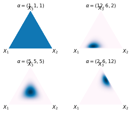
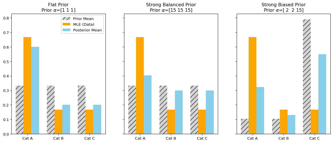
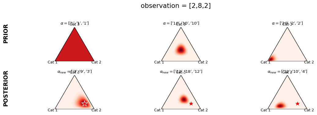
Illustration of Dirichlet Prior

Dirichlet prior adds a psuedo \(\alpha\) observations. (The observed data is [8,2,2])

Dirichlet as a multinomial distribution prior

Set up

• \(X = x_1,\dots,x_n\) are observations drawn from a Multinomial distribution with \(P=(p_1,\dots,p_K)\) and \(K\) classes.

Prior

A Dirichlet prior \(P(\textbf{p} \mid \mathbf{\alpha}) = \text{Dir}(\textbf{p} \mid \mathbf{\alpha}) = \frac{1}{\text{B}(\mathbf{\alpha})} \prod_{i=1}^K p_i^{\alpha_i - 1}\)

The probability of observing this data is

\[ \small p(X|p)= \frac{n!}{x_1!\dots x_k!}\prod_{j=1}^K p_j^{x_j} \propto \prod_{j=1}^K p_j^{x_j} \]

Using Bayes’ Rule, the posterior is proportional to the Likelihood times the Prior: \[ P(\textbf{p} \mid \textbf{X}, \mathbf{\alpha}) \propto P(\textbf{X} \mid \textbf{p}) P(\textbf{p} \mid \mathbf{\alpha}) \]

Dropping the constants (terms not involving \(\textbf{p}\)) to find the kernel:

\[ P(\textbf{p} \mid \mathbf{x}, \mathbf{\alpha}) \propto \left( \prod_{i=1}^K p_i^{x_i} \right) \left( \prod_{i=1}^K p_i^{\alpha_i - 1} \right) \]

Illustration

Thep posterior distribution has the kernel (functional form) of a Dirichlet distribution with updated parameters \(\mathbf{\alpha}'\):

\[ \begin{aligned} \mathbf{\alpha}' = (\mathbf{\alpha} + \textbf{x}) = (\alpha_1 + x_1, \alpha_2 + x_2, \dots, \alpha_K + x_K) \end{aligned} \]

Interpretation: The \(\alpha_i\) values act as “imaginary” observations seen before the experiment.

Interpretation of Dirichlet prior

	Categorical	Multinomial
Prior	Dirichlet	Dirichlet
Posterior	\(\prod_{k=1}^Kp_k^{n_k+\alpha_k-1}\)	\(\prod_{k=1}^Kp_k^{x_k+\alpha_k-1}\)
Posterior predictive	Categorical	Dirichlet-multinomial

• Interpretation:
  • Adding a Dirichlet prior is equivalent to adding \(\alpha\) pseudo-observations to the data.
  • As the number of observations increases, the influence of the prior decreases.

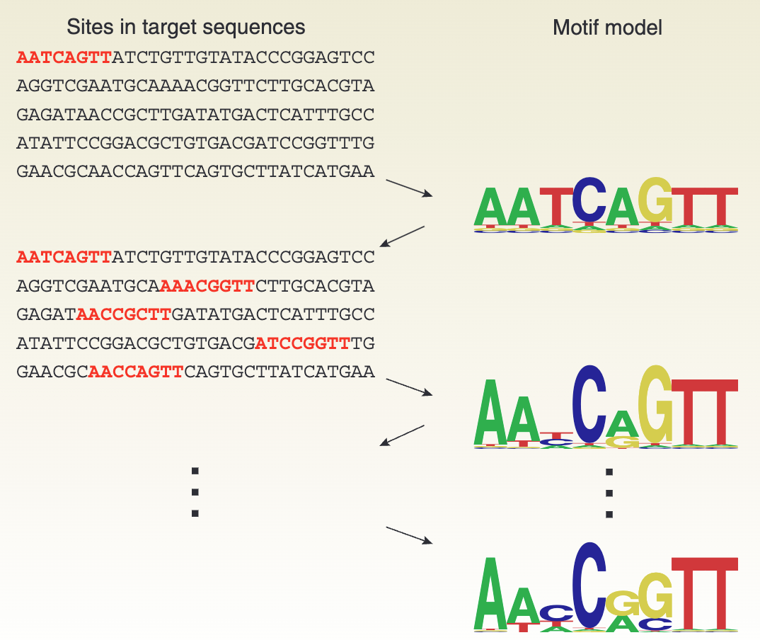
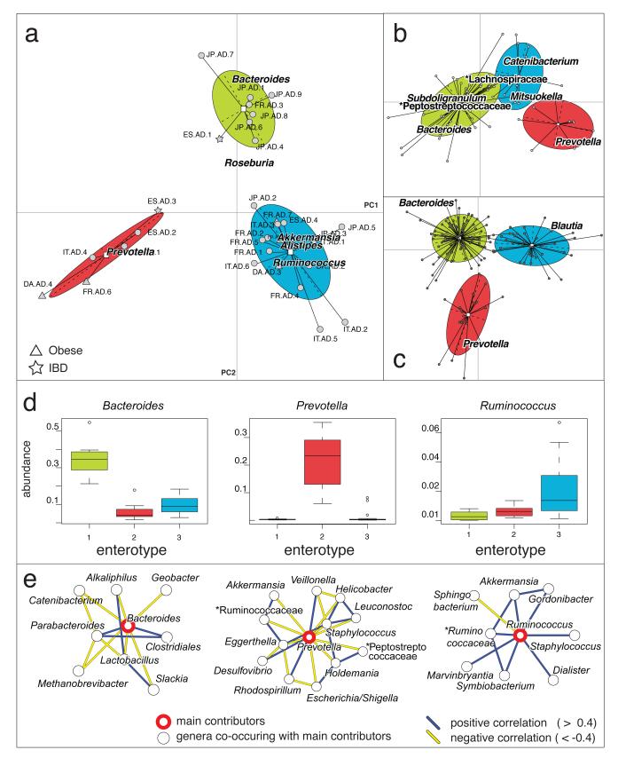
Application in bioinformatics

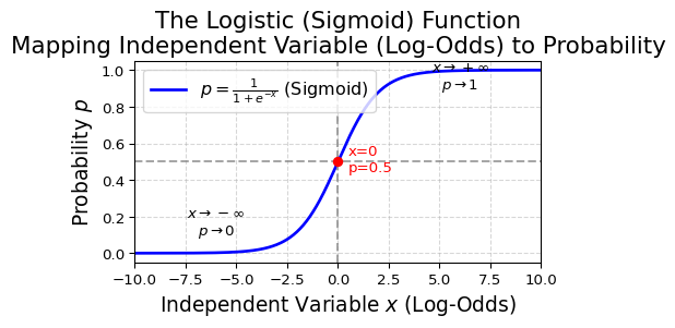
Motif discovery

Motif discovery from D’haeseleer (2006)

Metagenomics

Gut microbiome composition of different types from Arumugam et al. (2011)

Connection with linear regression (Optional)

Generalized linear model

Limitations of ordinary linear regression

• Count data (Multinomial/Poisson)
• Dichotomous or Multinomial outcomes (Bernoulli)
• Proportions (values between 0 and 1)

A generalized linear model (GLM) can model different kinds of data.

Components of GLM

• Random components
  • Identify \(Y\) and its distribution
• Systematic components
  • Linear predictor \(\alpha + \beta_1 x_1 + \dots + \beta_k x_k\)
• Link function
  • Given \(\mu=E(Y)\), the link function \(g(\cdot)\) satisfies \[g(\mu)=\alpha+\beta_1x_1+\dots+\beta_kx_k\]

Logistic regression

In logistic regression (binomial outcomes), the link function is

Logit link function
\[ \log\frac{p(x)}{1-p(x)}=\alpha+\beta x \]

Transform them back to get \(p(x)\)

\[ p(x)=\frac{e^{\alpha+\beta x}}{1+e^{\alpha+\beta x}} \]

For a dichotomous predictor \(x\) with values 0 and 1, \(\beta\) is the log odds ratio (\(\log(\text{OR})\)).

Discussion: if we model \(p(x)=\alpha+\beta x\), is it causing any trouble?

• Potential estimate for \(p(x)>1\) or \(p(x)<0\)

Multinomial logistic regression

• How do we compare multiple categories?
  • 1 vs. n
  • n vs. n
• There are \(k(k-1)/2\) pairs of comparisons, but actually, you only need \(k-1\) non-redundant comparisons.

Let the category \(K\) as the baseline, for each comparison of \(k = 1,\dots,k-1\)

Baseline-category logit model are \[ \log(\frac{p_k(x)}{p_K(x)})=\alpha_k+\beta_kx \quad k=1,\dots,K-1 \]

Interpretation of \(\beta\)

The model assumes \(\ln(\frac{p(x)}{1-p(x)})=\alpha+\beta x\), so for a given change \(\Delta x\),

The odds at \(x + \Delta x\) is

\[ \frac{p(x + \Delta x)}{1-p(x + \Delta x)}=\exp(\alpha+\beta(x+\Delta x)) = \exp(\alpha+\beta(x))\exp(\beta\Delta x) \]

The odds ratio (OR) for \(x\) is

\[ \text{OR}=\frac{\text{odds at}(x+\Delta x)}{\text{odds at}(x)}=\frac{\exp(\alpha+\beta(x+\Delta x))}{\exp(\alpha+\beta(x))} = \exp(\beta\Delta x) \]

• \(\beta\) is the change in the log odds when x increases by 1 unit.
• Confidence interval of OR is not symmetric to the mean.

How about alpha ?

Connections with contingency tables

Logistic regression v.s. Contingency table

	Logistic regression	Contingency table
Estimating	OR	OR
Test on esstimation	t-test/\(\chi^2\) test	Fisher’s exact test/\(\chi^2\) test

• Advantage of logistic regression
  • Controlling other confounders
• Estimating OR for continuous variables
• Compatible with multinomial outcomes

Back to the kidney stone example

In clinical practice, for stone diameters less than 2cm, doctors usually conduct PCNL, while open surgery is used for stone diameters of 2cm or greater.

Stone size	Treatment	Success	Fail
Small	OS	81	6
Small	PCNL	234	36
Large	OS	192	71
Large	PCNL	55	25

Model: (Success/Fail) ~ Stone size + Treatment

-- Log Odds Ratios & CI w/o Control Stone Size --
              2.5%  97.5%  Odds Ratio
Intercept     1.28   1.83        1.56
Treatment_OS -0.66   0.08       -0.29

-- Log Odds Ratios & CI with Control Stone Size  --
                  2.5%  97.5%  Odds Ratio
Intercept         1.60   2.27        1.94
Stone_Size_Large -1.73  -0.79       -1.26
Treatment_OS     -0.09   0.81        0.36

Connections to continuous variables

Ordinal logistic regression

For ordinal data (e.g., a scale with scores “No”, “Neutral”, and “Yes”), the following rules apply:

\[ P(x \leq k)=p(x=1) + \dots + p(x=k), \text{where } p(x\leq K) = 1 \]

Intuitively, we can think that the regression is measuring the same thing, but the cutoff for making decisions is different. So, we only need to estimate the cumulative logits:

\[ \log(\frac{p(x\leq j)}{p(x > j)}) =\alpha_j+\beta x \]

Ordinal logistic regression

Illustration: \(\alpha_{-1}=-3,\alpha_{0}=2, \beta=1.5\)

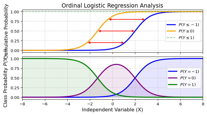
Implications

1. Finding cut-offs for different ordinal outcomes
2. If we extend to really continuous case, then we do not need that cut-offs to specific class

Bibliography

Arumugam, Manimozhiyan, Jeroen Raes, Eric Pelletier, Denis Le Paslier, Takuji Yamada, Daniel R Mende, Gabriel R Fernandes, et al. 2011. “Enterotypes of the Human Gut Microbiome.” Nature 473 (7346): 174–80.

D’haeseleer, Patrik. 2006. “How Does DNA Sequence Motif Discovery Work?” Nature Biotechnology 24 (8): 959–61.